Quick Introduction to CIMSS TC-Core

The CIMSS TC-Core product is an AI model of estimated surface windspeed in the TC inner vortex. The model is trained on twenty years of flight reconnaissance data matched with microwave and IR satellite imagery. In real-time deployment, the model uses this same satellite input, plus storm translation and shear, and produces a wind profile inside a ~150 km radius.

How to Read the Image Product

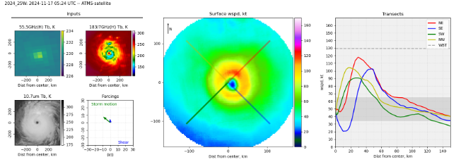
1. Inputs – These are the main input variables to the model. The 89 GHz image (for conical scanner data) or the 183 GHz image (for cross-track scanners) in the upper-right reveal intense convection and is the dominant data source because of its close association with eyewall structure. The 37 GHz image varies more with precipitation and provides a secondary input for TC structure. The infrared input (10.7 um, lower left) may also contribute eyewall structure information, especially if the eyewall is weak in the microwave images. The vector Forcings (lower right) help interpret the asymmetry in the wind profile product. In particular, storm motion is used both as an AI model input and as a post-processing data source.
2. Surface Windspeed – Surface windspeed is the full model product. The range is limited to approximately 150 km radius because this is also the approximate limit of the densest flight reconnaissance data. The image also contains four sample-transect lines to correspond to the profiles in the Transects plot. Note that the image center is not the position of the lowest winds. Rather, the image center is at the ARCHER center of the input microwave satellite imagery. This center position happens to be the most likely location to line up the peak winds along each transect for a good RMW reading, but with asymmetric winds, there is always a tradeoff in center fixing that is difficult to reconcile objectively.
3. Transects – The transects are radial wind profiles sampled through the 2D product. They are chosen to provide a straightforward aide in interpreting the critical wind radii at the product time. Also included here are a baseline reading of the working best track (WBT Vmax) for that time, and the raw model peak wind, explained later. Note that the minimum wind is rarely at distance = 0 on this plot, for reasons given immediately above.

Differences Between the Conical Scanner and Cross-Track Scanner Models

The differences in relevant channels between the conical microwave scanners and the cross-track scanners makes for interesting science but involves extra work for interpretation. The “183/7 GHz” (183+/-7 GHz) channel plays essentially the same role as the 89 GHz channel. On the other hand, the 55.5 GHz channel reveals the extent of upper tropospheric subsidence in the eye, which is a unique but indirect indicator of eyewall structure.

The conical and cross-track models are closely related in design but because of their unique data inputs they are developed as distinct and independent AI models. For this reason they may differ in their product output, and we are still working to evaluate these differences.

Important Surface Conversions

Before post-processing, the original model output is 700 hPa, storm-relative wind. It then undergoes three conversions to arrive at the final product shown here. First, it is converted to surface-level wind using the Franklin et al. (2003) conversion factors. Second, it is converted to earth-relative wind by adding the storm motion vector throughout the wind field. (Thus, the storm motion conversion is the main source of asymmetry in the wind product.) Third, the wind is normalized to the corresponding D-MINT model maximum surface wind estimate. This was found to be important because the original model shows good relative wind profiles, but less accurate absolute wind profiles. The normalization process thus combines the best features of both products.

Further Reading

Wimmers et al. (2024) describes the design of the original model, discusses performance characteristics across a range of TC structures, and analyzes product error.